77
Datasets
9,068
Samples
30
Signatures
Introduction
Prostate cancer
Prostate cancer (PCa) is the second most frequently diagnosed cancer in men worldwide, which accounts for 14.1% of the newly diagnosed cancer cases in 2020 [ GLOBOCAN ]. Localized PCa is a heterogeneous disease with highly variable clinical outcomes, which presents enormous challenges in the clinical management. The majority of patients with indolent PCa only require active surveillance, whereas patients with aggressive PCa require immediate local treatment. Comprehensive collection of transcriptomics data from large population cohorts is very critical for understanding the molecular biology of cancer, drug target identification and evaluation, and biomarker discovery for cancer diagnosis and prognosis, etc.
About PCaDB
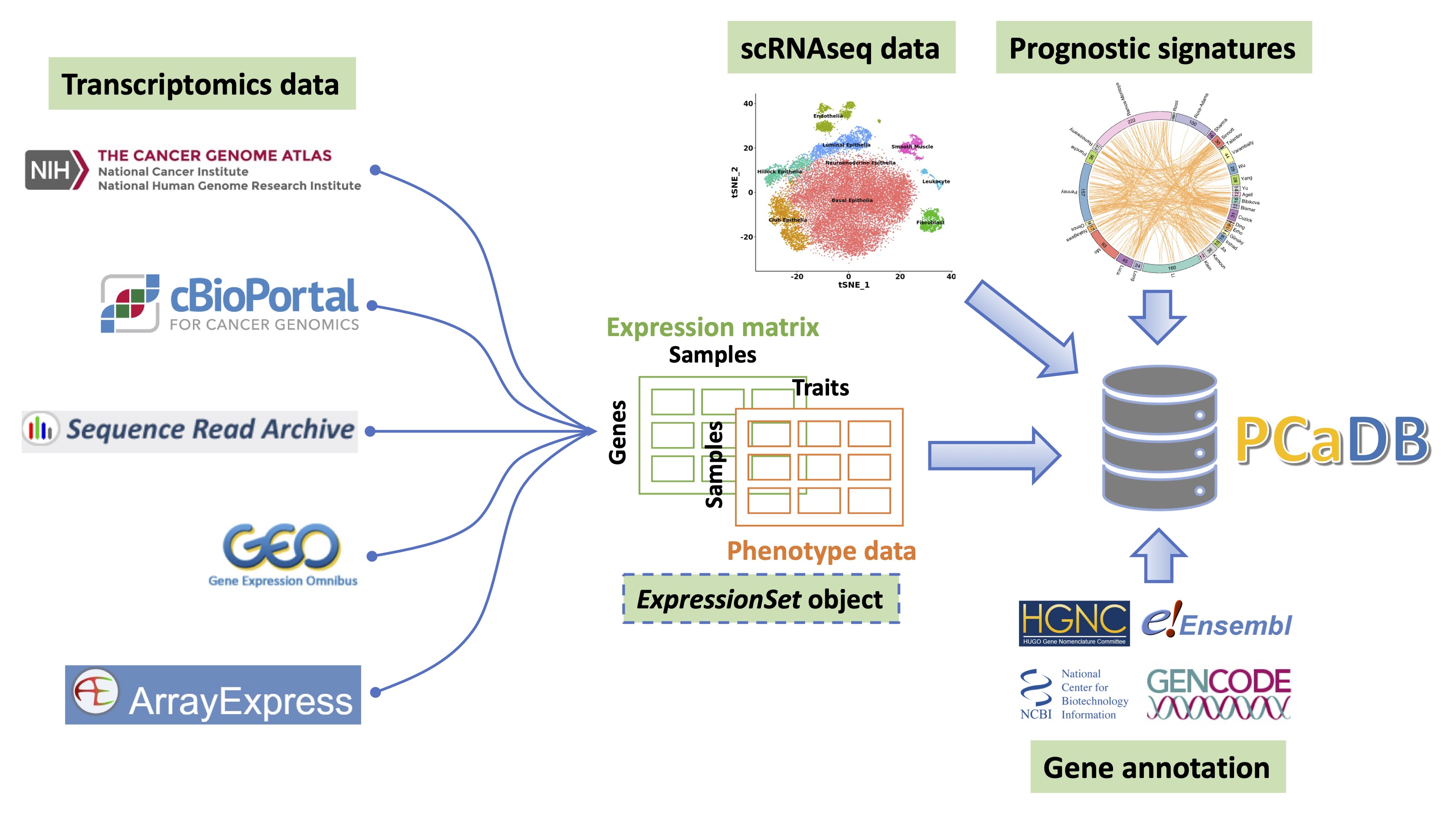
PCaDB is a comprehensive and interactive database for transcriptomes from prostate cancer population cohorts. We collected 77 transcriptomics datasets with 9,068 patient samples and a single-cell RNA-sequencing (scRNAseq) dataset with ~ 30,000 cells for normal human prostates from public data repositories. We also included a comprehensive collection of 30 published gene expression-based prognostic signatures in PCaDB. A standard bioinformatics pipeline is developed to download and process the expression data and sample metadata of the transcriptomics datasets.
PCaDB provides a user-friendly interface and a suite of data analysis and visualization modules for the comprehensive analysis of individual genes, prognostic signatures, and the whole transcriptomes to elucidate the molecular heterogeneity in PCa, understand the mechanisms of tumor initiation and progression, as well as develop and validate prognostic signatures in large independent cohorts.
Citation
Please cite the following publication: Li, R., Zhu, J., Zhong, W.-D., and Jia, Z. (2021) PCaDB - a comprehensive and interactive database for transcriptomes from prostate cancer population cohorts. bioRxiv, 10.1101/2021.06.29.449134.
https://doi.org/10.1101/2021.06.29.449134
Gene Expression in Different Sample Types
Kaplan Meier Survival Analysis (Forest Plot)
(Low- and high-expression groups were separated by median values)
Kaplan Meier Survival Curve
(Low- and high-expression groups were separated by median values)
tSNE Plot
UMAP Plot
Prognostic Signatures
Gene Expression Signatures for Prostate Cancer Prognosis
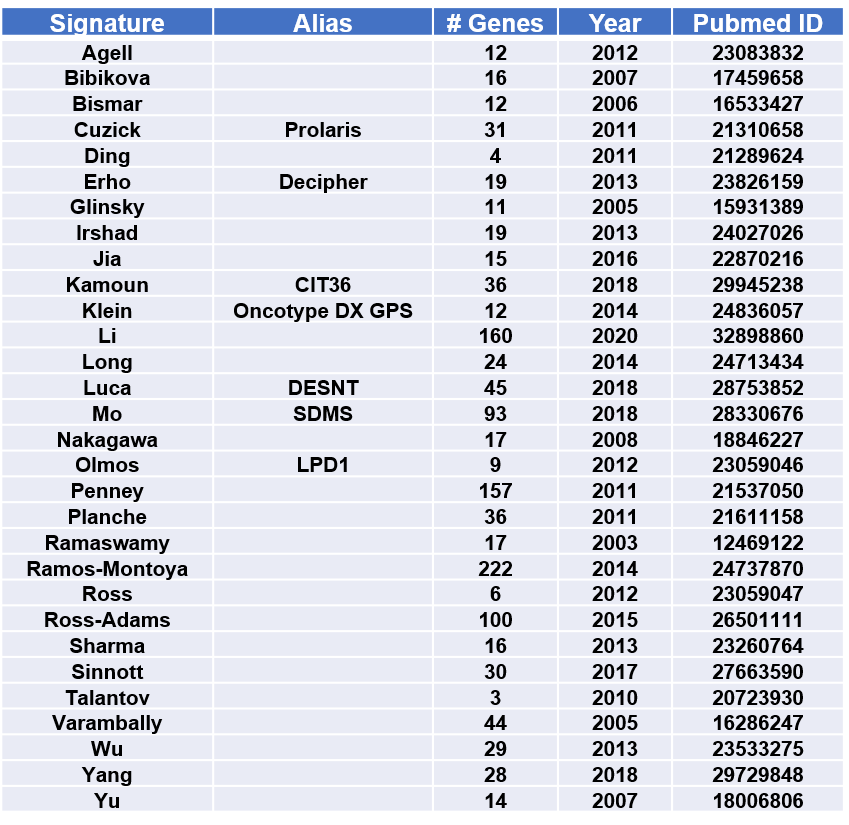
An inclusive collection of 30 published gene expression-based prognostic signatures for prostate cancer is included in PCaDB. The performances of the signatures have been investigated in the study [ Comprehensive evaluation of machine learning models and gene expression signatures for prostate cancer prognosis using large population cohorts ]. Comprehensive characterization of the signatures can be further performed in PCaDB.
List of genes in the selected prognostic signature
Volcano Plot of Differentially Expressed Genes in the Signatures
(|Fold Change| > 2 & FDR < 0.01)
List of Differentially Expressed Genes in the Signatures
(|Fold Change| > 2 & FDR < 0.01)
KM Survival Analysis of RFS for Common Genes in 3 or more Signatures
(Low- and high-expression groups were separated by median values)
KM Survival Analysis of RFS for All the Signature Genes
(Low- and high-expression groups were separated by median values)
Functional Enrichment Analysis of Signature Genes
Bar Plot of the Top 30 Enriched Pathways
Bubble Plot of the Top 30 Enriched Pathways
Comparison of the performances of the prognostic signatures
C Index
Hazard Ratio (KM)
Area Under the ROC Curve
C Index
Hazard Ratio of KM analysis
Time-dependent AUC
Transcriptome Analysis
Select a Transcriptome Dataset
Summary
GEO/ArrayExpress Accession: SRA Accession: cBioPortal:
Data Preprocessing:
Sample Type
PSA
Gleason Pattern
BCR Status
Time to BCR
2D Principal Component Analysis
3D Principal Component Analysis
Select the Case/Control Groups for Comparison:
Volcano Plot of Differentially Expressed Genes
List of Differentially Expressed Genes
Univariate Kaplan Meier (KM) Survival Analysis
(Low- and high-expression groups were separated by median values)
Univariate Cox Proportional-Hazards (CoxPH) Survival Analysis
Multivariate Cox Proportional-Hazards (CoxPH) Survival Analysis
* Clinical factors that are used for multivariate CoxPH survival analysis in each dataset
(Y: included; N: not included)
Prognostic Model
Kaplan Meier Survival Analysis in the Training Dataset
(Low- and high-risk groups were separated by median values)
Kaplan Meier Survival Analysis in the Validation Datasets
PCaDB Pipeline
Details about PCaDB pipeline
- Overview
- SRA RNAseq data
- TCGA RNAseq data
- cBioPortal RNAseq data
- GEO/ArrayExpress microarray data
- Sample metadata model
- Single-cell RNAseq data
- Gene annotation
Overview
A suite of bioinformatics pipelines has been developed to download, process, and harmonize the transcriptomics data from multiple public data repositories, including Sequence Read Archive (SRA), Genomic Data Commons (GDC)/The Cancer Genome Atlas (TCGA), cBioPortal, Gene Expression Omnibus (GEO), and ArrayExpress.
In general, among the 77 datasets in PCaDB, (i) 17 datasets from SRA and 37 datasets from GEO/ArrayExpress with the raw FASTQ or CEL files, respectively, were reprocessed using the PCaDB pipeline; (ii) read count data for the TCGA-PRAD project was downloaded from GDC; (iii) normalized data such as RPKM/FPKM values for the 6 RNAseq datasets in cBioPortal were downloaded directly; and (iv) normalized intensities for the other 16 microarray datasets without raw data were downloaded from GEO. For RNAseq data from TCGA and SRA, the raw count data is normalized using the Trimmed Mean of Mvalues (TMM) method implemented in the R package
edgeR[1], and lowly-expressed genes with logCPM < 0 in more than 50% of samples are filtered out prior to any downstream analysis. For the Affymetrix microarray data with raw CEL files in GEO/ArrayExpress, the Robust Multichip Average (RMA) method implemented in the R package
oligo[2] was used for data normalization. For a small proportion of the datasets that only have normalized data provided in the public data repository, the methods for data processing described in the original papers were carefully inspected to make sure that appropriate processing methods had been used. All the gene expression values are in log2 scale. In PCaDB, the Ensembl gene identifiers are used for all the datasets. If multiple probes/genes matched to the same Ensembl ID, only the most informative one with the maximum interquartile range (IQR) for the gene expression is used for this Ensembl ID.
A comprehensive metadata model has been developed to harmonize the sample metadata (phenotype data) from the public repositories. The ExpressionSet object has been created for each dataset, allowing users to easily download both the gene expression data and harmonized metadata for advanced downstream analyses.
A single-cell RNAseq dataset from normal human prostae tissue [3] was downloaded from GUDMAP (https://www.gudmap.org/), allowing the investigation of a gene of interest at the single-cell level.
30 prognostic signatures for prostate cancer were obtained from a comprehensive study evaluating the machine learning models and gene expression signatures for prostate cancer prognosis using large population cohorts [4]. The 10 datasets used in that study were all included in the PCaDB database.
We also systematically organized the gene annotation information from HGNC, Ensembl, NCBI, and Gencode to facilitate the query of individual genes and the cross-dataset anlaysis.
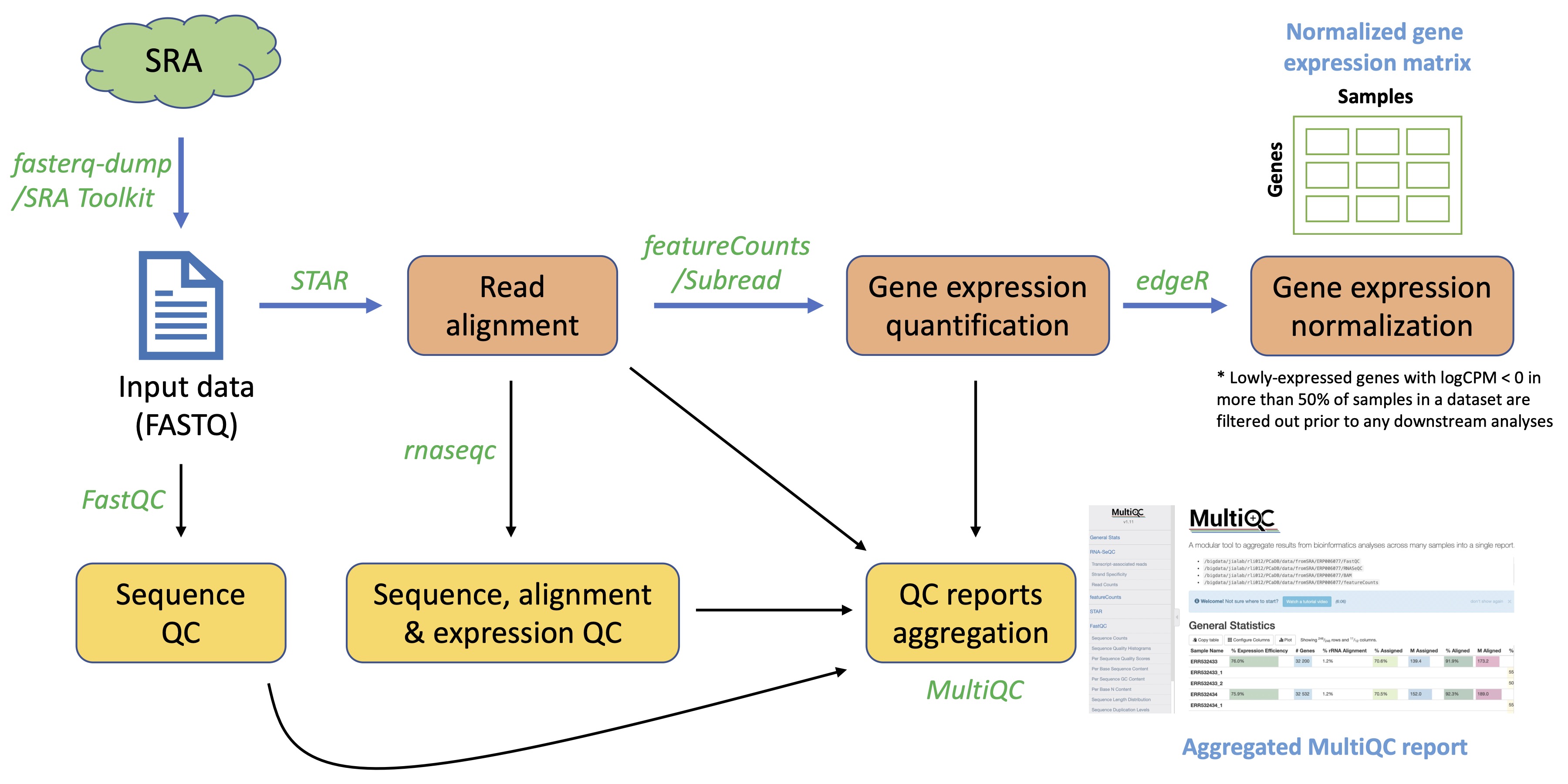
Overview of the pipeline is shown in the figure below and details about the pipeline are described in the sub-sections.
SRA RNAseq data
For the 17 RNAseq datasets in SRA, the
fasterq-dumptool in
SRA Toolkit (2.10.8)[5] was used to download and convert SRA data into FASTQ format. The
FastQC (v0.11.5)[6] tool was used for a comprehensive quality control of the sequencing data, including base sequence quality, GC content, overrepresented sequences, and adapter content, etc. Read trimming was not performed since a few benchmark studies have demonstrated that it's not necessary to remove adapter sequences or low-quality bases before alignment because the adapter sequences can be efficiently removed by read aligner via 'soft-cipping' and the low-quality bases can be rescued by the aligner [ref]. The most widely used aligner for RNAseq data -
STAR (2.7.9a)[7] was adopted to align the sequencing reads to the reference genome
GRCh38 (primary assembly)
based on the
GENCODE (release 38)
gene annotation [8]. The 2-pass mapping was performed for each sample separately.
STARwill perform the 1st pass mapping and then automatically extract junctions and insert them into the genome index, and, finally, re-align all reads in the 2nd mapping pass [ref]. The BAM files generated from the alignment step were sorted using
samtools (v1.9)[9]. The
featureCountsprogram [10] in the
Subread (2.0.3)package was used for gene expression quantification to generate the count matrix. Only read pairs that were uniquely mapped to the exonic regions were quantified. The count data was finally normalized using the Trimmed Mean of Mvalues (TMM) method implemented in the R package
edgeR, and lowly-expressed genes with logCPM < 0 in more than 50% of samples were filtered out prior to any downstream analysis. To generate a more comprehensive QC report, we used the
rnaseqc (v2.4.2)tool [11] to characterize the quality of the RNA, sequencing data, alignment, and expression profile of each sample. Over 70 QC metrics can be computed by
rnaseqc, including rRNA rate and exonic/intronic/intergenic rate, etc. Finally, an aggregated QC report can be generated using
MultiQC[12] to display the QC metrics from multiple bioinformatics analyses, including
FastQC,
STAR,
featureCounts, and
rnaseqc.
All the scipts for SRA RNAseq data processing are publicly available in Github:
https://github.com/rli012/PCaDB.
TCGA RNAseq data
The raw sequencing data in TCGA was processed using a similar pipeline (
TCGA mRNA Analysis Pipeline) as what is being used by PCaDB for SRA RNAseq data processing (described above). The sequencing reads were aligned to the human reference genome
GRCh38
using the 2-pass mapping implemented in
STAR (2.4.2a)based on
GENCODE (release22)
for gene annotation. The major difference between TCGA workflow and PCaDB workflow is that
HTSeq (0.6.1p1)[13] was used by TCGA for gene expression quantification, whereas
featureCounts/Subread (2.0.3)is adopted by PCaDB. The HTSeq-Counts data for The Cancer Genome Atlas Prostate Adenocarcinoma (TCGA-PRAD) project is publicly available in Genomic Data Commons (GDC), which can be downloaded and processed directly by a series of functions in the R package
GDCRNATools[14] to generate the count matrix. The count data was also normalized using the Trimmed Mean of M values (TMM) method implemented in the R package
edgeR. Silimarly, lowly-expressed genes with logCPM < 0 in more than 50% of samples were filtered out prior to any downstream analysis.
Below is the script for downloading, preprocessing, and organizing data from TCGA-PRAD.
cBioPortal RNAseq data
Although transcriptomics data for multiple PCa cohorts are included in cBioPortal, the cBioPortal data are usually not used in PCaDB, unless the raw data are not available in any of the other data repositories, because only the normalized RNAseq data are provided in cBioPortal, which may not be suitable for some of the downstream analyses. e.g., the FPKM/RPKM values are not recommended for differential expression analysis.
For the 6 cBioPortal RNAseq datasets included in PCaDB, normalized gene expression data (FPKM/RPKM values) were downloaded directly from cBioPortal. Log2 transformation may be performed if it hadn't been done and the gene symbols/entrez ids were all converted to Ensembl IDs. If multiple genes matched to the same Ensembl ID, only the most informative one with the maximum interquartile range (IQR) for the gene expression is used for this Ensembl ID.
A custom script below is used to curate cBioPortal data.
GEO/ArrayExpress microarray data
Among the 38 datasets generated using the Affymetrix arrays (e.g., Affymetrix Human Exon 1.0 ST Array, Affymetrix Human Gene 2.0 ST Array, Affymetrix Human Genome U133A Array, and Affymetrix Human Genome U133 Plus 2.0 Array, etc.), 37 of them with the raw CEL files were reprocessed by the PCaDB pipeline. The R package
GEOquery[15] was used to download the CEL files and the Robust Multichip Average (RMA) method implemented in the R package
oligowas used for background correction, quantile normalization, and log2 transformation. The annotation package downloaded from the
Brainarray database(
Version 24.0.0; GENCODE release 32
) was used for probe/gene annotation [16].
The only Affymetrix microarray dataset that was not reprocessed by our PCaDB pipeline is the CPC-Gene dataset (GSE107299). The reason was because that this dataset was generated based on two different Affymetrix arrays: Affymetrix Human Gene 2.0 ST Array (Batch 1,3,4,5) and Affymetrix Human Transcriptome Array 2.0 (Batch 2) with a batch effect. Therefore, the batch-corrected normalized data was downloaded directly from GEO. Likewise, the normalized intensities for the 15 microarray datasets generated using other technologies (e.g., Illumina HumanHT-12 V3.0 Expression Beadchip and Agilent-012391 Whole Human Genome Oligo Microarray G4112A, etc.) without raw data in GEO were downloaded directly from the repository using
GEOquery. The methods for data processing described in the original papers were carefully inspected to make sure that appropriate processing methods had been used. Log2 transformation may be performed on the normalized data if it hadn't been done and the probe/gene ids were all converted to Ensembl IDs. If multiple probes/genes matched to the same Ensembl ID, only the most informative one with the maximum interquartile range (IQR) for the gene expression is used for this Ensembl ID.
Sample metadata model
Harmonization of sample metadata is very critical for the management and downstream analysis of omics data. In PCaDB, a comprehensive metadata model is built to harmonize the most important sample and clinical information across the datasets. A total of 33 key fields/traits are included:
sample_id
,
patient_id
,
tissue
,
batch
,
platform
,
sample_type
,
age_at_diagnosis
,
ethnicity
,
race
,
clinical_stage
,
clinical_t_stage
,
clinical_n_stage
,
clinical_m_stage
,
pathological_stage
,
pathological_t_stage
,
pathological_n_stage
,
pathological_m_stage
,
preop_psa
,
gleason_primary_pattern
,
gleason_secondary_pattern
,
gleason_tertiary_pattern
,
gleason_group
,
gleason_score
,
time_to_death
,
os_status
,
time_to_bcr
,
bcr_status
,
time_to_metastasis
,
metastasis_status
,
risk_group
,
treatment
,
additional_treatment
, and
pcadb_group
.
The
pcadb_group
column in each dataset was manually created with the group information that are of the most interests to end users depending on the availability, such as normal, primary tumor, and metastatic castration-resistant prostate cancer (CRPC); pre-androgen-deprivation therapy (ADT) and post-ADT samples; samples from the peripheral zone and the transcription zone of the prostate; samples from the European Americans and African Americans, etc.
The phenotypic values were also standardized, especially for the sample type field. For example,
tumor, tumour, primary, localized,etc. were all labeled as
Primary, whereas
normal, adjacent, benign,etc. were all labeled as
Normal.
The pipeline for metadata harmonization is very similar for data from different repositories. The differences are just the ways to download and retrieve the data.
For sample metadata from the TCGA-PRAD project, the XML files with the clinical information of the patients were downloaded and organized using the R package
GDCRNATools. Some clinical features, such as preoperative prostate-specific antigen (PSA) level, which were not available in the Genomic Data Commons (GDC) data portal were retrieved from Broad GDAC Firehose (https://gdac. broadinstitute.org/).
The phenotype data of the datasets in GEO was retrieved using our in-house web tool -
WebGEO(under development) based on the R package
GEOquery, which allows querying and downloading the sample metadata of a dataset in seconds. In case users are interested in downloading phenotype data programmatically using
GEOquery, the script is also provided below
Most of the SRA datasets (14 out of 17) also have corresponding GEO accessions, thus the sample metadata for these datasets were also retrieved from GEO using
WebGEO. For the 3 remaining SRA datasets that do not have corresponding GEO accessions, the metadata (SraRunTable) were downloaded directly from SRA.
Most of the SRA datasets (14 out of 17) also have corresponding GEO accessions, thus the sample metadata for these datasets were also retreived from GEO using
WebGEO. For the 3 remaining SRA datasets that do not have corresponding GEO accessions, the metadata (SraRunTable) were downloaded directly from SRA.
Clinical data for the 6 cBioPortal RNAseq datasets were manually downloaded from the portal, and sample metadata (.sdrf.txt file) for the 4 ArrayExpress datasets were downloaded using
wget.In addition, the original publications were carefully reviewed to further ensure the accuracy and comprehensiveness of the sample metadata for each dataset in PCaDB.
Single-cell RNAseq data
The Seurat object of the single-cell RNAseq data can be directly downloaded from
GUDMAP. The normalized gene expression matrix, cell type annotation, as well as the TSNE and UMAP coordiantes were included in an R list object in the PCaDB database.
For details about the scRNAseq data analysis, such as data processing, data normalization, tSNE and UMAP analyses, etc., please refer to the original study [3].
Gene annotation
Gene annotation information were downloaded from the official websites/FTPs of HGNC [17], Ensembl [18], NCBI [19], and GENCODE [8], and a comprehensive pipeline was created to map the gene IDs from different resources to facilitate the query of individual genes and the cross-dataset anlaysis. The harmonized gene annotation data has been deposited in PCaDB and can be easily downloaded on the
Download
page (PCaDB_Gene_Annotation.RDS).
References
[1] Robinson, M.D., McCarthy, D.J. and Smyth, G.K. (2010). edgeR: a Bioconductor package for differential expression analysis of digital gene expression data. Bioinformatics, 26(1), 139-140.
[2] Carvalho, B.S. and Irizarry, R.A. (2010). A framework for oligonucleotide microarray preprocessing. Bioinformatics, 23(14), 1846-1847.
[3] Henry, G.H., Malewska, A., Joseph, D.B., Malladi, V.S., Lee, J., Torrealba, J., Mauck, R.J., Gahan, J.C., Raj, G.V., Roehrborn, C.G., Hon, G.C., MacConmara, M.P., Reese, J.C., Hutchinson, R.C., Vezina, C.M. and Strand, D.W. (2018). A Cellular Anatomy of the Normal Adult Human Prostate and Prostatic Urethra. Cell reports, 25(12), 3530-3542.
[4] Li, R., Zhu, J., Zhong, W.-D., and Jia, Z. (2021) Comprehensive evaluation of machine learning models and gene expression signatures for prostate cancer prognosis using large population cohorts. bioRxiv. https://doi.org/10.1101/2021.07.02.450975
[5] SRA Toolkit Development Team. Available online at: https://trace.ncbi.nlm.nih.gov/Traces/sra/sra.cgi?view=software
[6] Andrews, S. (2010). FastQC: a quality control tool for high throughput sequence data. Available online at: http://www.bioinformatics.babraham.ac.uk/projects/fastqc
[7] Dobin, A., Davis, C.A., Schlesinger, F., Drenkow, J., Zaleski, C., Jha, S., Batut, P., Chaisson, M. and Gingeras, T.R., (2013). STAR: ultrafast universal RNA-seq aligner. Bioinformatics, 29(1), pp.15-21.
[8] Frankish, A., Diekhans, M., Jungreis, I., Lagarde, J., Loveland, J.E., Mudge, J.M., Sisu, C., Wright, J.C., Armstrong, J., Barnes, I. and Berry, A., (2021). GENCODE 2021. Nucleic acids research, 49(D1), pp.D916-D923.
[9] Li, H., Handsaker, B., Wysoker, A., Fennell, T., Ruan, J., Homer, N., Marth, G., Abecasis, G. and Durbin, R., (2009). The sequence alignment/map format and SAMtools. Bioinformatics, 25(16), pp.2078-2079.
[10] Liao, Y., Smyth, G.K. and Shi, W., (2014). featureCounts: an efficient general purpose program for assigning sequence reads to genomic features. Bioinformatics, 30(7), pp.923-930.
[11] Graubert, A., Aguet, F., Ravi, A., Ardlie, K.G. and Getz, G., (2021). RNA-SeQC 2: efficient RNA-seq quality control and quantification for large cohorts. Bioinformatics.
[12] Ewels, P., Magnusson, M., Lundin, S. and Käller, M., (2016). MultiQC: summarize analysis results for multiple tools and samples in a single report. Bioinformatics, 32(19), pp.3047-3048.
[13] Anders, S., Pyl, P.T. and Huber, W., (2015). HTSeq—a Python framework to work with high-throughput sequencing data. bioinformatics, 31(2), pp.166-169.
[14] Li, R., Qu, H., Wang, S., Wei, J., Zhang, L., Ma, R., Lu, J., Zhu, J., Zhong, W.-D. and Jia, Z. (2018). GDCRNATools: an R/Bioconductor package for integrative analysis of lncRNA, miRNA and mRNA data in GDC. Bioinformatics, 34(14), 2515-2517.
[15] Davis, S. and Meltzer, P.S. (2007). GEOquery: a bridge between the Gene Expression Omnibus (GEO) and BioConductor. Bioinformatics, 23(14), 1846-1847.
[16] Dai, M., Wang, P., Boyd, A.D., Kostov, G., Athey, B., Jones, E.G., Bunney, W.E., Myers, R.M., Speed, T.P., Akil, H. and Watson, S.J., (2005). Evolving gene/transcript definitions significantly alter the interpretation of GeneChip data. Nucleic acids research, 33(20), pp.e175-e175.
[17] Tweedie, S., Braschi, B., Gray, K., Jones, T.E., Seal, R.L., Yates, B. and Bruford, E.A., (2021). Genenames. org: the HGNC and VGNC resources in 2021. Nucleic Acids Research, 49(D1), pp.D939-D946.
[18] Howe, K.L., Achuthan, P., Allen, J., Allen, J., Alvarez-Jarreta, J., Amode, M.R., Armean, I.M., Azov, A.G., Bennett, R., Bhai, J. and Billis, K., (2021). Ensembl 2021. Nucleic acids research, 49(D1), pp.D884-D891.
[19] Sayers, E.W., Beck, J., Bolton, E.E., Bourexis, D., Brister, J.R., Canese, K., Comeau, D.C., Funk, K., Kim, S., Klimke, W. and Marchler-Bauer, A., (2021). Database resources of the national center for biotechnology information. Nucleic acids research, 49(D1), p.D10.
Download
Transcriptome Datasets
Prognostic Signatures
Gene Annotation
Tutorial
Details about the tutorial
- Query a gene of interest
- Prognostic signature evaluation
- Transcriptomics data analysis
- Data download
Query a gene of interest
1.1. Overview
Users can query a gene of interest by typing the Ensembl ID, Entrez ID, or HGNC approved symbol and alias symbol in the 'Search a gene' field and selecting the gene from the dropdown list. The general information about the gene and some useful external links to the databases such as ENSEMBL, HGNC, and NCBI for more detailed description of the gene, Genotype-Tissue Expression (GTEx) and Human Protein Atlas (HPA) for the gene expression pattern in different human tissues, and Kyoto Encyclopedia of Genes and Genomes (KEGG) for the pathways that the gene involves in are provided (Figure 1-1).
A suite of advanced analyses and visualizations can be interactively performed for the selected gene, including:
(1) Gene expression in different sample types
(2) Survival analysis of relapse-free survival (RFS)
(3) Gene expression analysis at the single-cell level
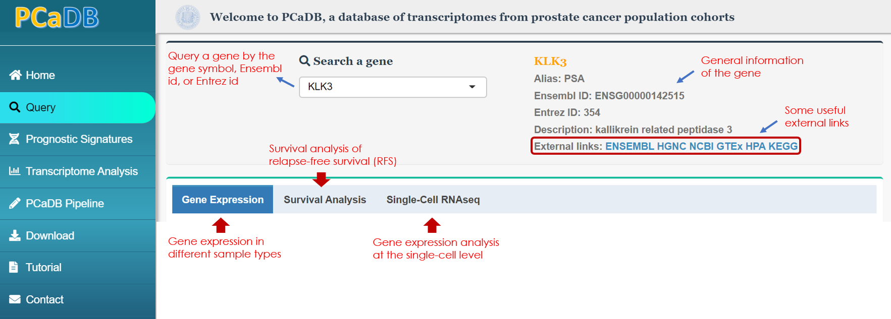
Figure 1-1. Query a gene of interest
1.2. Gene expression in different sample types
Users can select a dataset from the dropdown list and a boxplot will be generated to visualize the gene expression levels in different samples, such as primary tumor, tumor-adjacent normal, or metastatic tumor samples, depending on the availability of the data in the selected dataset (Figure 1-2)
The pipelines used for gene expression data normalization have been described in the 'PCaDB Pipeline' tab. In general, (i) for RNAseq data from TCGA and SRA, the counts per million mapped reads (CPM) vaules are used; (ii) for microarray data from GEO and ArrayExpress, the normalized intensity values are used; and (iii) for the normalized RNAseq data downloaded directly from cBioPortal, the fragments/reads per kilobase of transcript per million mapped reads (FPKM/RPKM) values are used. All the gene expression values are in log2 scale. In PCaDB, the Ensembl gene identifiers are used for all the datasets. If multiple probes/genes matched to the same Ensembl ID, only the most informative one with the maximum interquartile range (IQR) for the gene expression is used for this Ensembl ID.
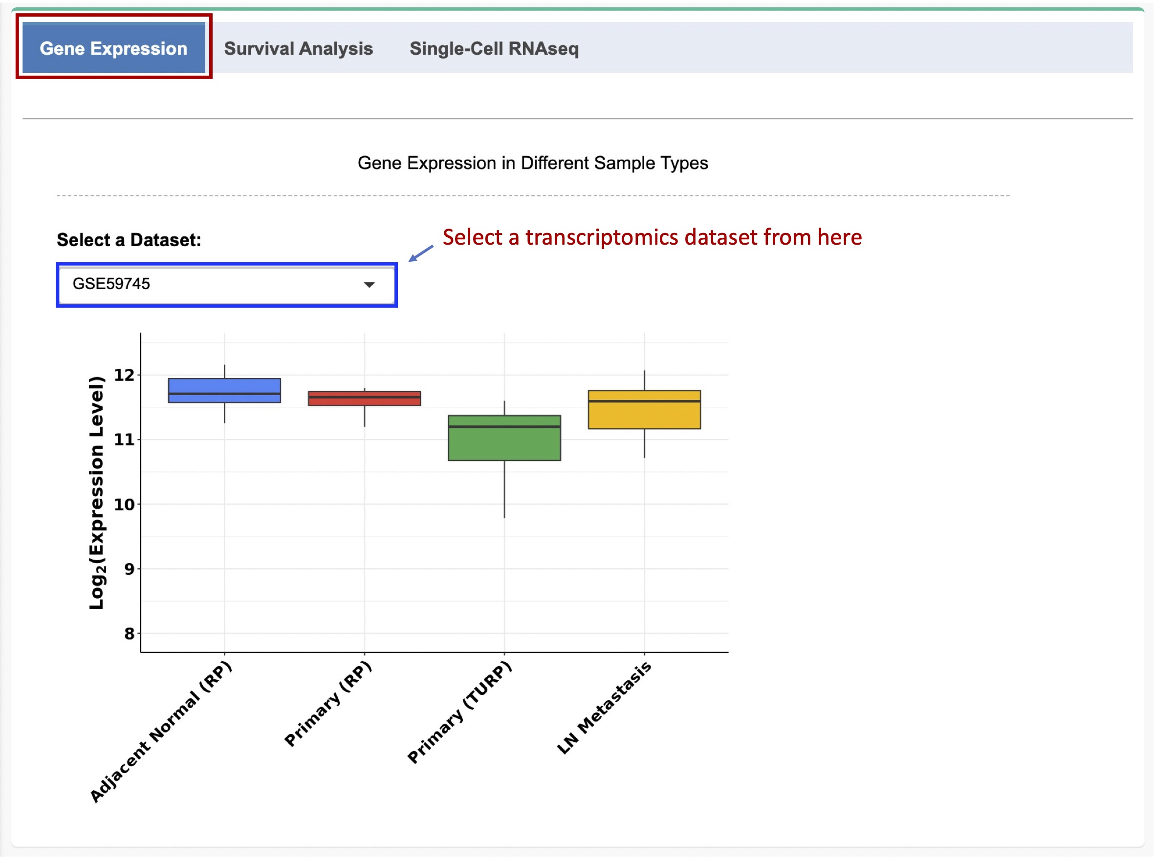
Figure 1-2. Gene expression in different sample types
1.3. Survival analysis of relapse-free survival (RFS)
Kaplan Meier (KM) survival analysis of relapse-free survival (RFS) for the selected gene can be performed in the 10 datasets with 1,558 primary tumor samples from PCa patients with the data of biochemical recurrence (BCR) status and follow up time after definitive treatment.
The patients in each dataset are dichotomized into low- and high-expression groups based on the median expression value of the selected gene. KM analysis is performed using the R package
survivalto estimate the hazard ratio (HR) and 95% confidence intervals (CIs). The log-rank test is used to compare the two survival curves and calculate the p value.
A forest plot with the result from the survival analysis, including the numbers of samples, hazard ratios (HRs), 95% confidence intervals (CIs), and p values across all the datasets, will be generated. The KM survival curve for each dataset will also be plotted (Figure 1-3).
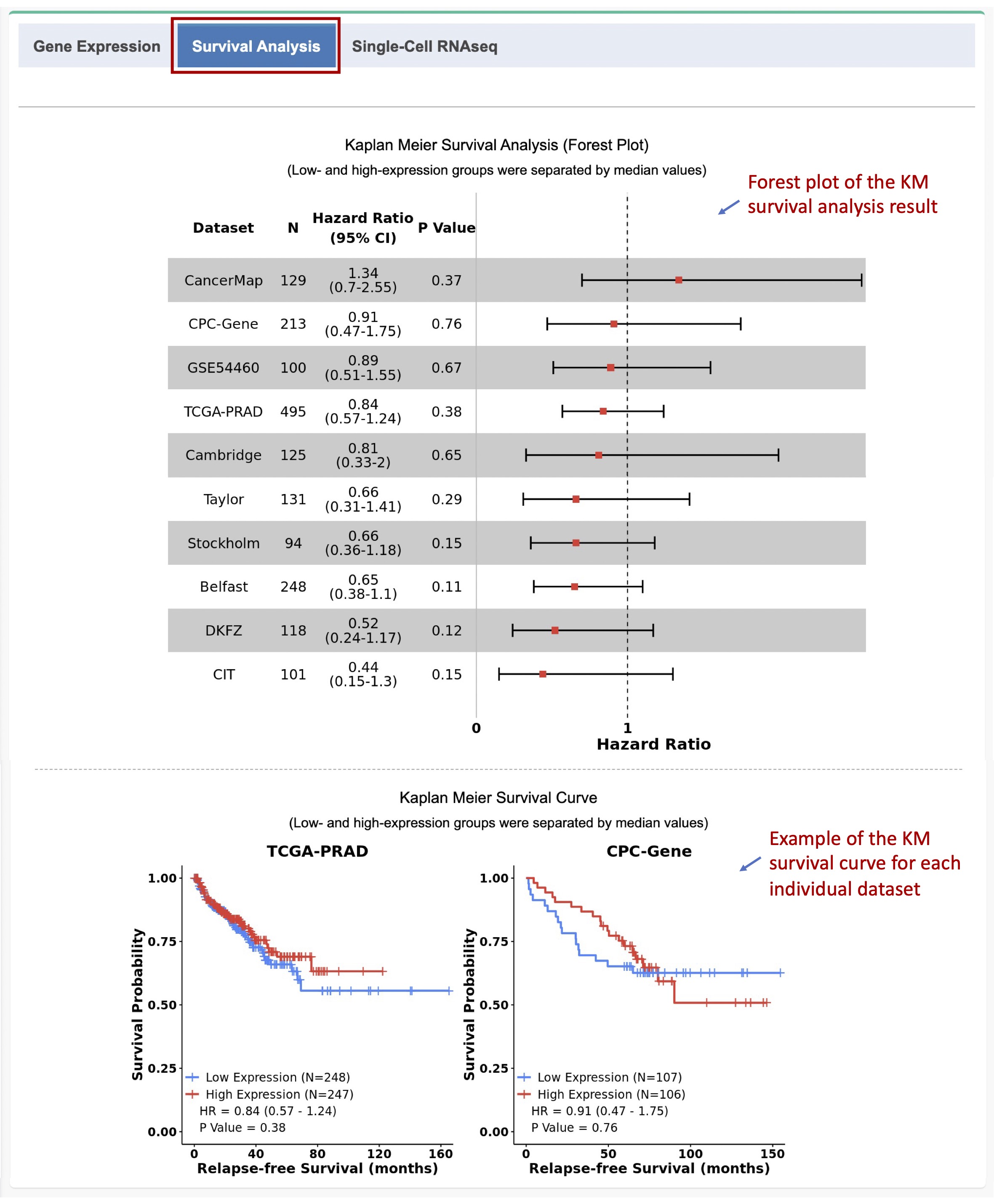
Figure 1-3. Forest plot and KM survival curves
1.4. Gene expression analysis at the single-cell level
The expression pattern of the selected gene in different cell types from normal human prostate, including basal, luminal, neuroendocrine (NE), club, and hillock epithelia, endothelia, leukocyte, fibroblast, and smooth muscle, can be visualized using the uniform manifold approximation and projection (UMAP) plot and t-distributed stochastic neighbor embedding (t-SNE) plot, violin plot, and bubble plot with the average gene expression and percent of cells expressed for each cell type (Figure 1-4). The data used in this module was downloaded directly from GUDMAP (https://www.gudmap.org/chaise/record/#2/RNASeq:Study/RID=W-RAHW).
For details about the scRNAseq data analysis, such as data processing, data normalization, tSNE and UMAP analyses, etc., please refer to the orignial study:
Henry, Gervaise H., et al. A cellular anatomy of the normal adult human prostate and prostatic urethra. Cell reports 25.12 (2018): 3530-3542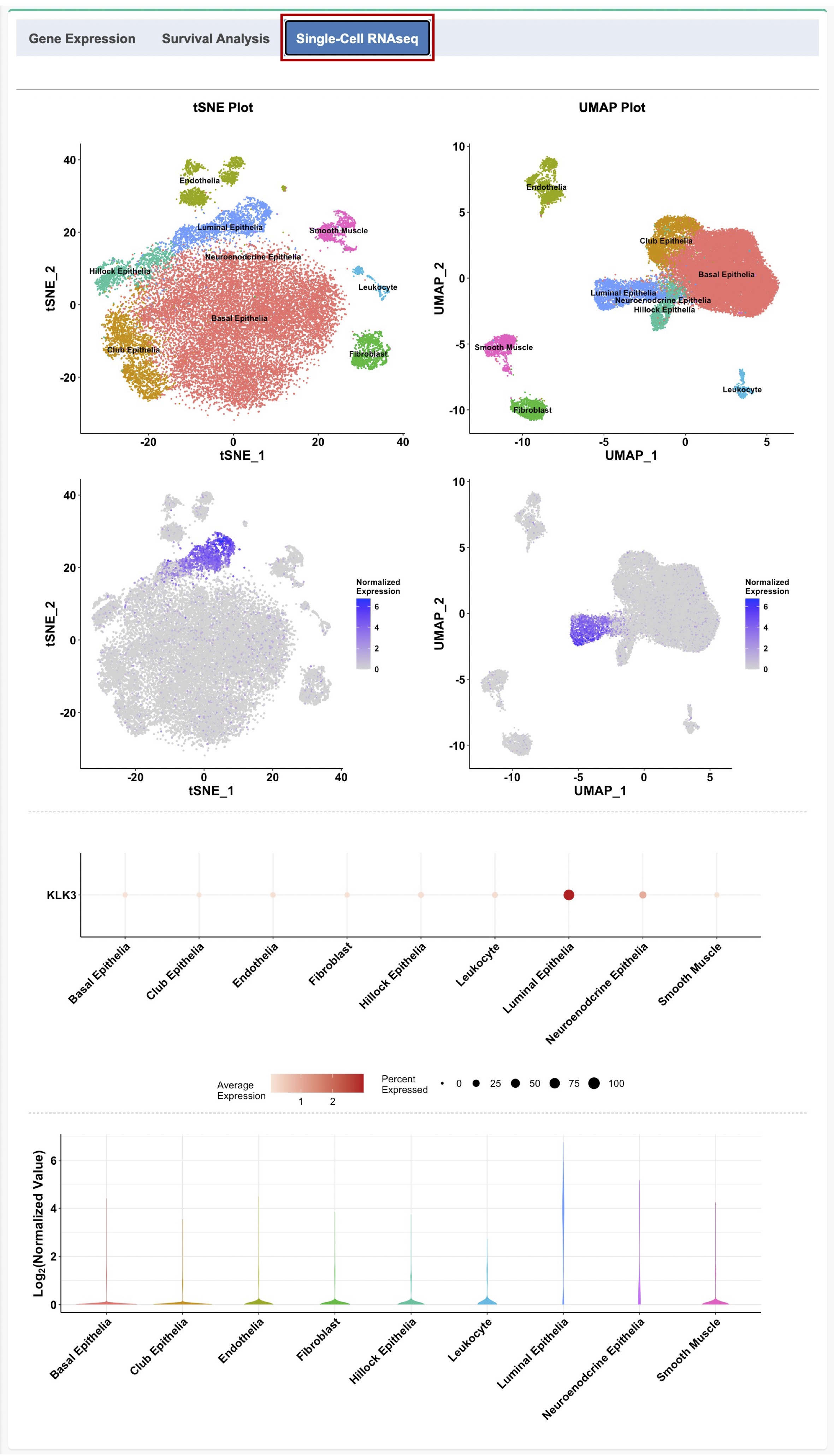
Figure 1-4. tSNE plot, UMAP plot, bubble plot, and violin plot to visualize the gene expression pattern at the single-cell level
Prognostic signature evaluation
2.1. Overview
A comprehensive evaluation of the prognostic performances of 30 published signatures was performed in a previous study and we included all those signatures in the PCaDB database, allowing for a more detailed characterization of the signatures (Figure 2-1), including:
(1) List of signature genes
(2) Differential expression analysis of the signature genes
(3) KM Survival analysis of RFS for the signature genes
(4) Pathway analysis of the signature genes
(5) Evaluation of the performances of the prognostic signatures
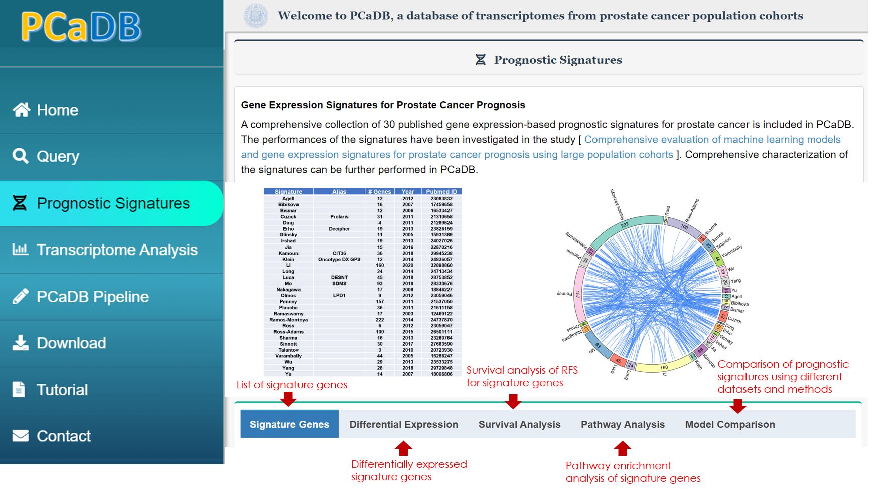
Figure 2-1. Overview of modules for prognostic signature evaluation
2.2. List of signature genes
The list of genes in a prognositc signature can be viewed by selecting the signature from the dropdown list. A comprehensive pipeline was created to convert the gene IDs/symbols reported in the orignial publication to the Ensembl IDs and HGNC gene symbols. We also did a manual inspection very carefully to double check the ambiguous signature genes.
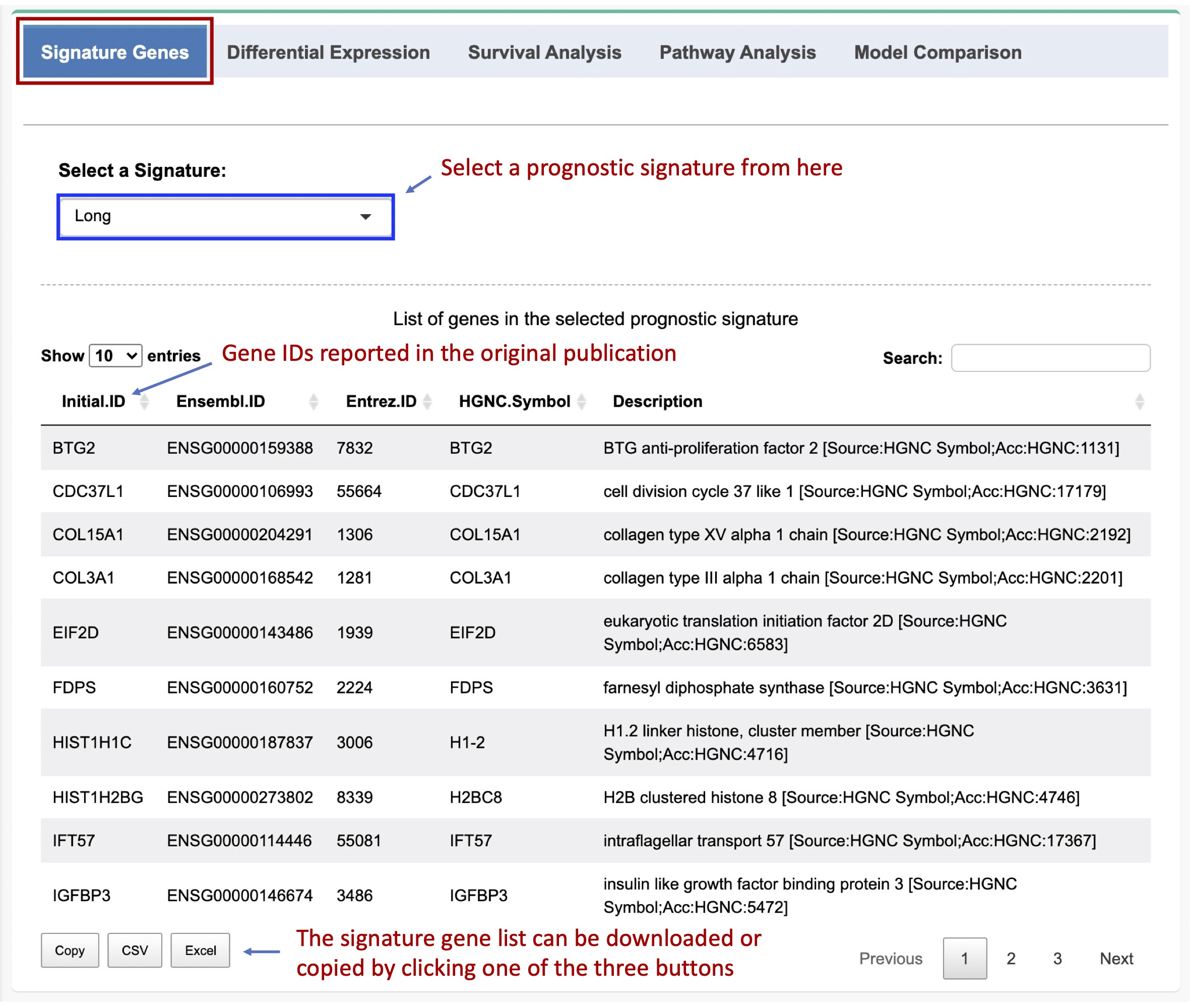
Figure 2-2. Th list of genes in the selected signature
2.3. Differential expression analysis of the signature genes
The DE analysis of all signature genes between primary tumor and tumor-adjacent normal samples can be performed using the R package
limmain multiple datasets with certain sample types. The normalized gene expression data in log2 scale is used as input. i.e., for RNAseq data from TCGA and SRA, the raw count data is normalized using the Trimmed Mean of Mvalues (TMM) method implemented in the R package
edgeR, followed by
voomtransformation using
limma, which is more powerful especially when the library sizes are quite variable between samples. Lowly-expressed genes (logCPM < 0 in more than 50% of samples) are filtered out before any downstream analysis. A linear model will then be fitted to estimate the fold changes and standard errors for each gene, followed by empirical Bayes smoothing. The differential expression analysis for Affymetrix microarray data is very similar to that for RNAseq data, except that the Robust Multichip Average (RMA) normalized intensity in log2 scale is fitted to the linear model. For some other datasets, the normalized data provided by the original studies are used as input for differential expression analysis.
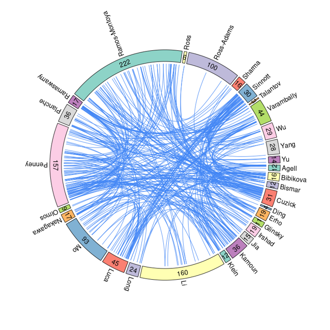
A volcano plot will be generated to visualize the DE analysis result. Only differentially expressed genes (DEGs) in >= 3 signatures are labeled in the volcano plot. A data table will also be created to list the DEGs. The log2(fold change), BH-adjusted p value (FDR), the number of signatures, and the names of the signatures are reported in the table (Figure 2-3).
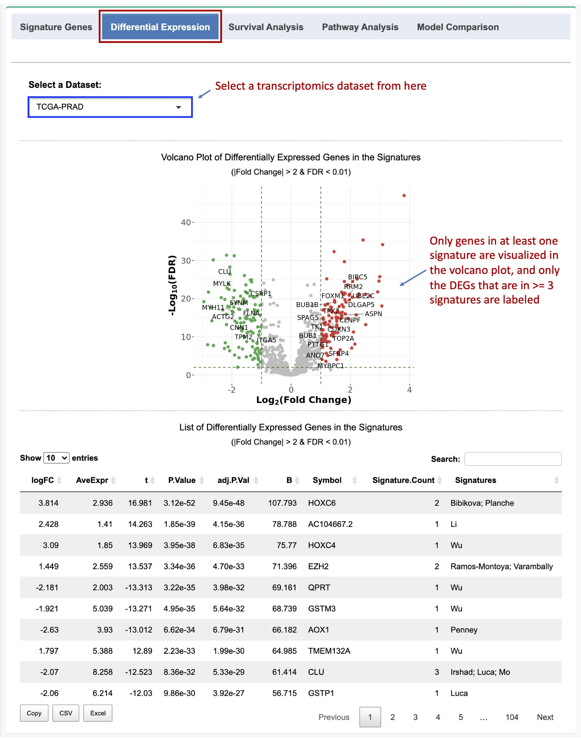
Figure 2-3. Differential expression analysis of the signature genes
2.4. KM Survival analysis of RFS for the signature genes
Kaplan Meier (KM) survival analysis of relapse-free survival (RFS) for the signature genes can be performed in the 10 datasets with 1,558 primary tumor samples from PCa patients with the data of biochemical recurrence (BCR) status and follow up time after definitive treatment.
The patients in each dataset are dichotomized into low- and high-expression groups based on the median expression value of the signature gene. KM analysis is performed using the R package
survivalto estimate the hazard ratio (HR) and 95% confidence intervals (CIs). The log-rank test is used to compare the two survival curves and calculate the p value.
A forest plot for the common genes in 3 or more signatures and a data table with the survival analysis result for all the signature genes are generated. In the data table, the hazard ratios (HRs), 95% confidence intervals (CIs), nominal p values, and BH-adjusted p values (FDRs), as well as the number of signatures and names of the signatures are reported (Figure 2-4).
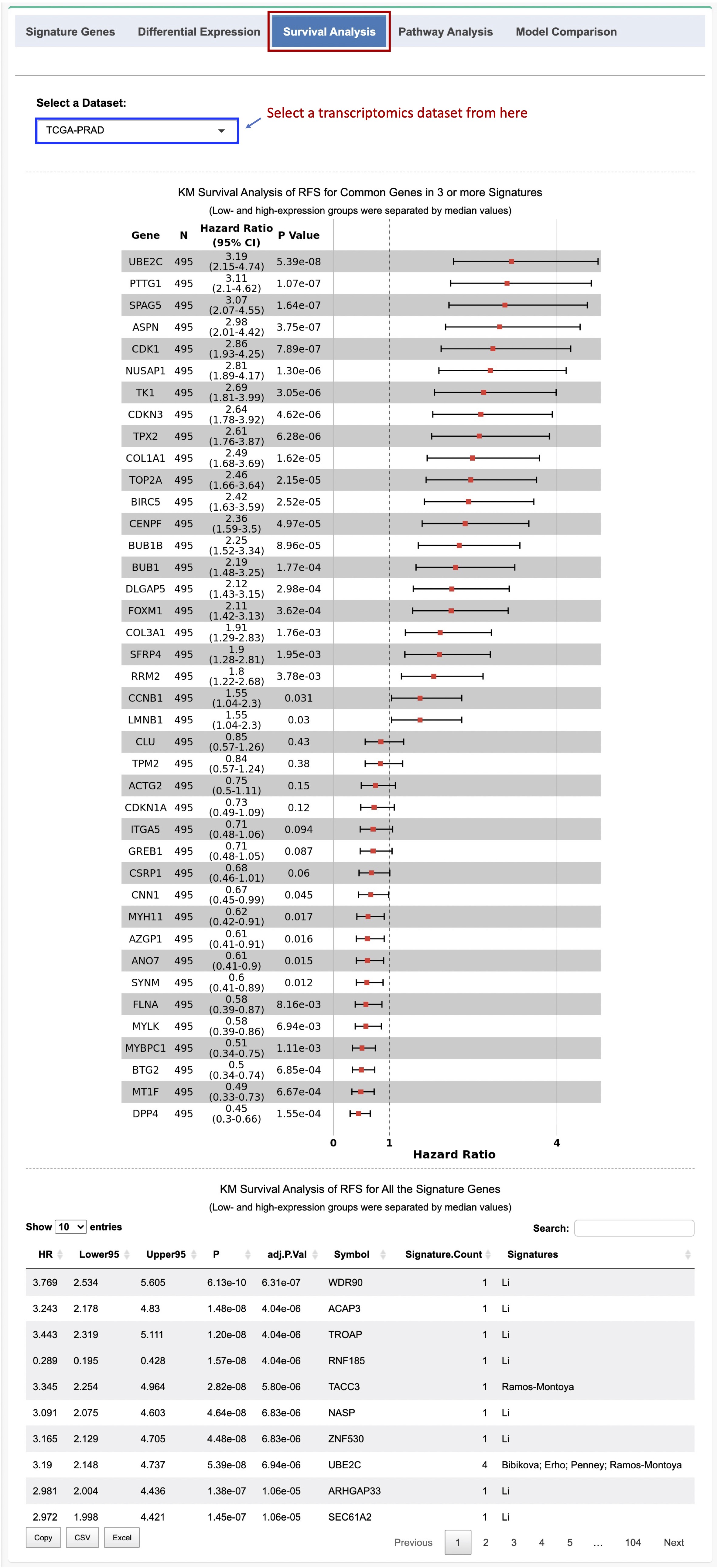
Figure 2-4. KM Survival analysis of RFS for the signature genes
2.5. Pathway analysis of the signature genes
Functional enrichment analysis of the signature genes can be performed using the R package
clusterProfilerin PCaDB based on hypergeometric test. Users can select a gene list from the dropdown list for the enrichment analysis. A gene list could consist of genes in an individual signature, common genes in at least 2, 3, or 4 signatures, and all the 1,042 signature genes. Pathways or Gene sets with < 10 genes or > 500 genes are excluded. Benjamini-Hochberg (BH) is used for multiple testing correction.
PCaDB supports functional enrichment analysis with many pathway/ontology knowledgebases, including:
(1) KEGG: Kyoto Encyclopedia of Genes and Genomes
(2) REACTOME
(3) DO: Disease Ontology
(4) NCG: Network of Cancer Gene
(5) DisGeNET
(6) GO-BP: Gene Ontology (Biological Process)
(7) GO-CC: Gene Ontology (Cellular Component)
(8) GO-MF: Gene Ontology (Molecular Function)
(9) MSigDB-H: Molecular Signatures Database (Hallmark)
(10) MSigDB-C4: Molecular Signatures Database (CGN: Cancer Gene Neighborhoods)
(11) MSigDB-C4: Molecular Signatures Database (CM: Cancer Modules)
(12) MSigDB-C6: Molecular Signatures Database (C6: Oncogenic Signature Gene Sets)
A data table is produced to summarize the significantly enriched pathways/ontologies in descending order based on their significance levels, as well as the number and proportion of enriched genes and the gene symbols in each pathway/ontology term.
'Count'is the number of genes shared between the input gene list and pathway/gene set;
'List Total'is the total number of genes in the input gene list;
'Pop Hits'is the number of genes in the pathway/gene set; and
'Pop Total'is the total number of genes in the pathway/gene set database, e.g., KEGG, GO, and REACTOME, etc.
The top enriched pathways/ontologies (based on the BH-adjusted p value) are visualized using both bar plot and bubble plot.
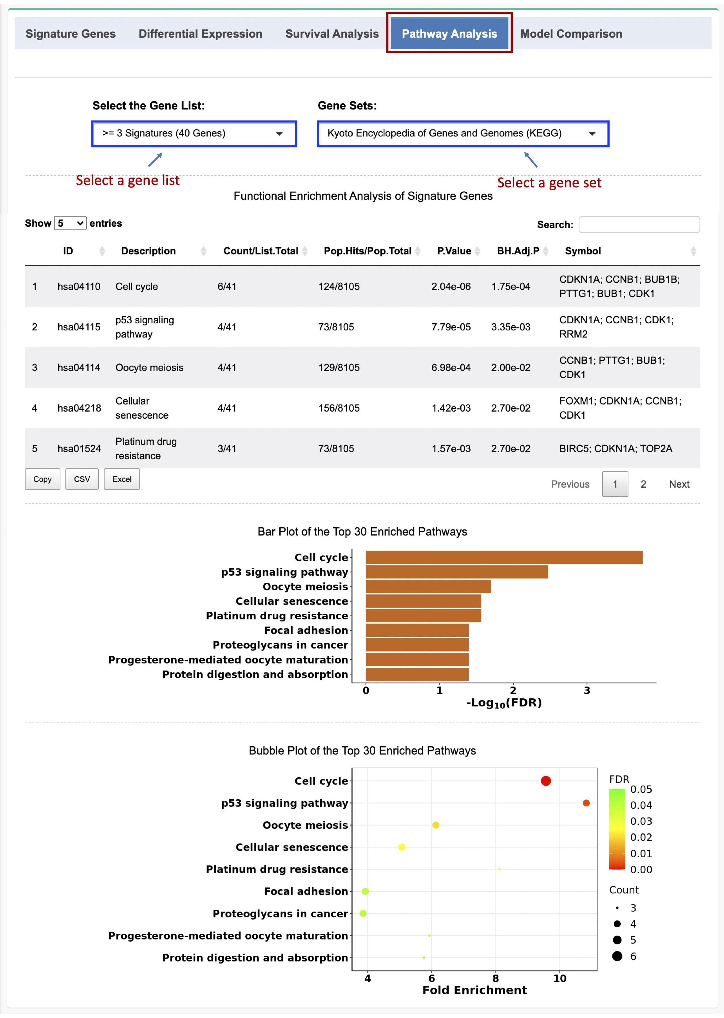
Figure 2-5. Pathway analysis of the signature genes
2.6. Evaluation of the performances of the prognostic signatures
A comprehensive evaluation of the performances of the published prognostic signatures can be performed in PCaDB using different survival analysis algorithms and different training and test datasets.
If a given signature is selected, a prognostic model can be developed using the expression data of the signature genes in the selected training dataset and the selected survival analysis method. The risk score of each patient in the test datasets will be computed based on the model.
For the intra-dataset comparison, 10-fold CV was used for model evaluation, whereas for the inter-dataset comparison, one dataset was treated as the training set and the other datasets were used as the test datasets at a time.
Three metrics including the concordance index (C-index), time-dependent receiver operating characteristics (ROC) curve, and hazard ratio (HR) estimated by the KM survival analysis are used to assess the prognostic power for the signature based on the independent test cohorts. Forest plots are used to visualize the results, while data tables with more detailed results are also provided.
For details about the machine learning algorithms, prognostic model training and testing, as well as the calculation of C index, AUC, and HR, etc., please refer to the orignial study:
Li R, Zhu J, Zhong W-D, Jia Z. Comprehensive evaluation of machine learning models and gene expression signatures for prostate cancer prognosis using large population cohorts. bioRxiv. 2021 (https://doi.org/10.1101/2021.07.02.450975)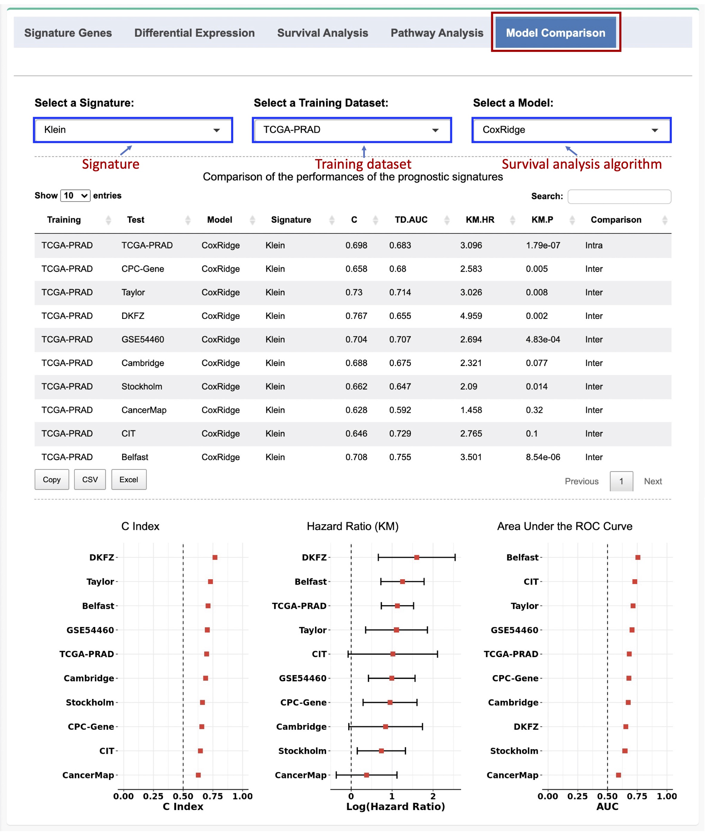
Figure 2-6. Evaluation of the prognostic performances of an individual signature
Users can also select ‘All Signatures’ from the dropdown list to perform a comprehensive analysis to compare and rank the prognostic abiligies of all the signatures in each individual test set based on the three metrics.
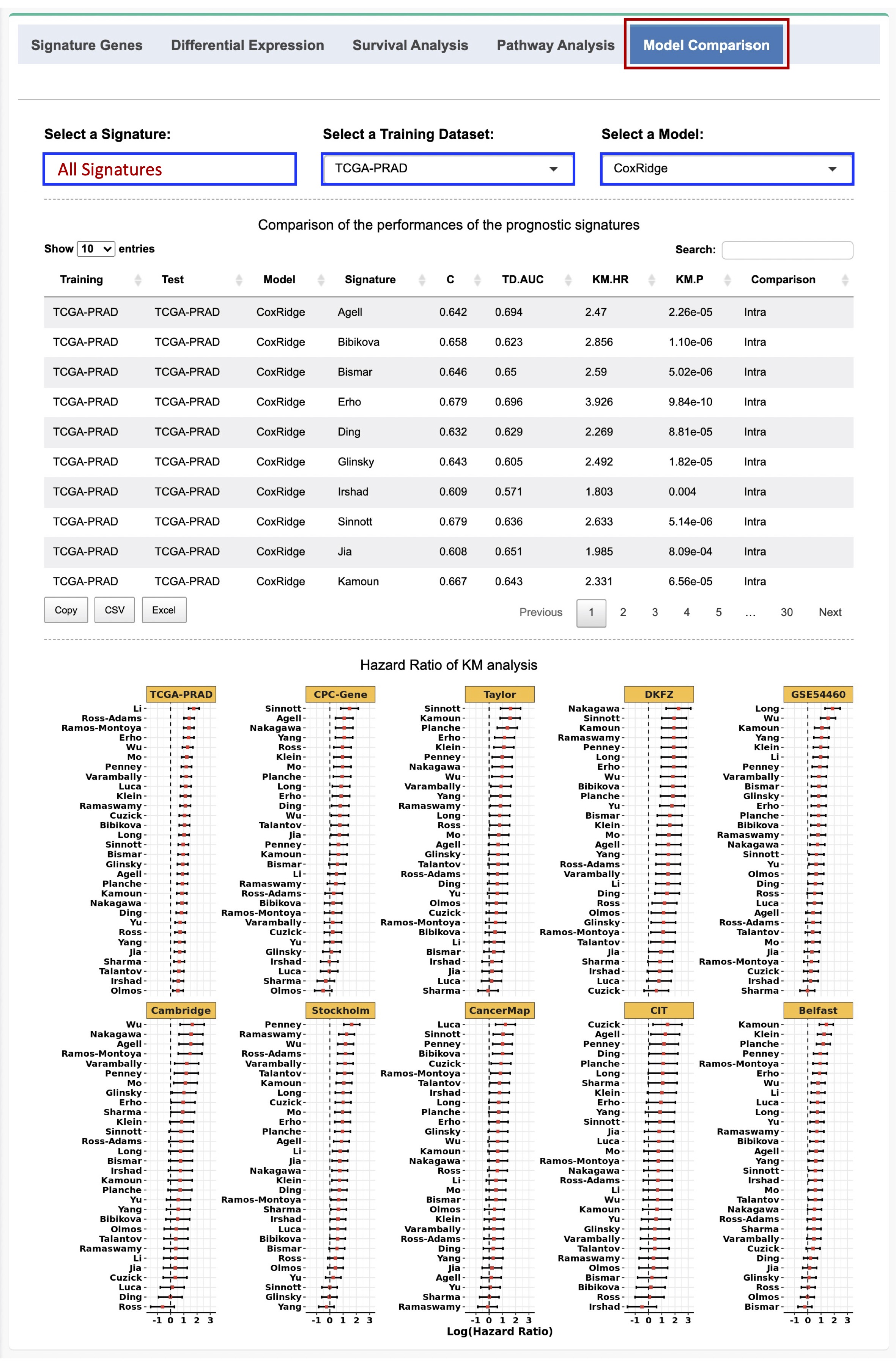
Figure 2-7. Evaluation of the prognostic performances of all the signatures
Transcriptomics data analysis
3.1. Overview
More advanced and comprehensive analyses can be performed at the whole-transcriptome level in PCaDB, allowing users to identify DEGs associated with tumor initiation and progression, identify biomarkers associated with clinical outcomes (i.e., BCR), as well as develop and validate gene expression-based signatures and models for PCa prognosis (Figure 3-1). The whole-transcriptome level analysis includes:
(1) Summary of the dataset
(2) Dimensionality reduction
(3) Differential gene expression analysis
(4) KM and CoxPH survival analyses of RFS (only for the first 10 datasets with the information of time to BCR)
(5) Development and validation of a new prognostic model (only for the first 10 datasets with the information of time to BCR)
Figure 3-1. Overview of whole-transcriptome data analysis
3.2. Summary of the dataset
When a transcriptomics dataset is selected, the summary of the dataset including platform, data processing pipeline, and the available metadata, such as sample type, preoperative PSA, Gleason score, BCR status, and time to BCR, will be displayed automatically (Figure 3-2).
Figure 3-2. Summary of the dataset
3.3. Dimensionality reduction
Principal component analysis (PCA) can be performed using the whole transcriptome profiling (lowly-expressed genes with logCPM < 0 in 50% of samples are filtered out for RNAseq data) in the selected dataset. The normalized gene expression data is rescaled by z-score standardization and the
prcompfunction in R is used for PCA analysis. The 2D or 3D interactive plot based on the first two or three principal components, respectively, will be generated for visualization (Figure 3-3).
Figure 3-3. Principal component analysis
3.4. Differential gene expression analysis
PCaDB has included transcriptomics data from a wide spectrum of sample types, which allows differential expression analysis between many different types of samples, such as the comparisons between prostate tissue from healthy donor, tumor-adjacent normal tissue, primary tumor and advanced tumor, non-metastatic castration-resistant prostate cancer (CRPC) vs. metastatic CRPC, CRPC at different sites (lymph node, bone, liver, lung, etc.), perineural invasion (PNI) tumor vs. non-PNI tumor, normal and tumor samples between African Americans vs. European Americans, tumor samples collected pre-androgen-deprivation therapy (ADT) vs. post-ADT, ADT responsive vs. castration resistant, etc.
The R package
limmais used to identify DEGs in PCaDB. The normalized gene expression data in log2 scale is used as input. i.e., for RNAseq data from TCGA and SRA, the raw count data is normalized using the Trimmed Mean of Mvalues (TMM) method implemented in the R package
edgeR, followed by
voomtransformation using
limma, which is more powerful especially when the library sizes are quite variable between samples. Lowly-expressed genes (logCPM < 0 in more than 50% of samples) are filtered out before any downstream analysis. A linear model will then be fitted to estimate the fold changes and standard errors for each gene, followed by empirical Bayes smoothing. The differential expression analysis for Affymetrix microarray data is very similar to that for RNAseq data, except that the Robust Multichip Average (RMA) normalized intensity in log2 scale is fitted to the linear model. For some other datasets, the normalized data provided by the originial studies are used as input for differential expression analysis. Benjamini-Hochberg (BH) is used for multiple testing correction.
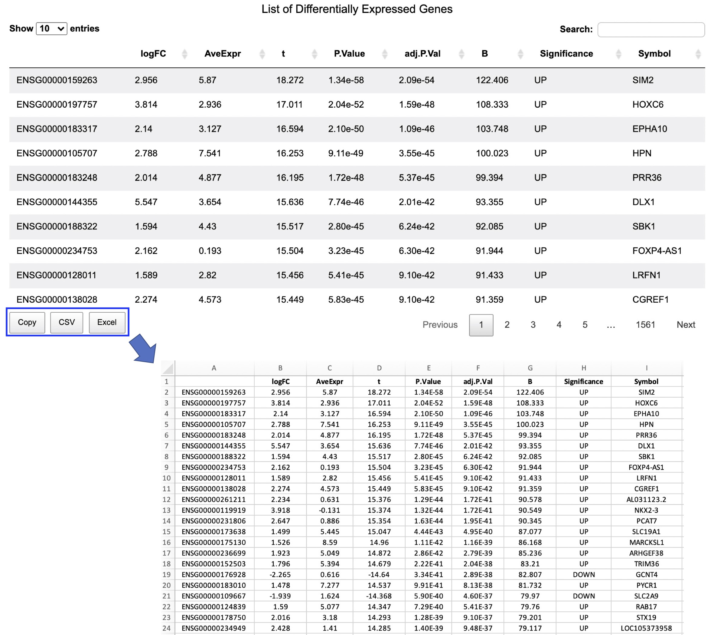
A volcano plot will be generated to visualize the DE analysis result. By default, BH-adjusted p value (FDR) < 0.01 and absolute fold change > 2 are used as the thresholds for determining DEGs. A data table will also be created to list the DE analysis result. The ensembl id, log2(fold change), average expression across all the samples, t statistics, nornimal p value, BH-adjusted p value (FDR), B statistics, gene expression regulation (Up: significantly up-regulated; Down: significantly down-regulated; NS: not significant), and gene symbol are reported in the table (Figure 3-4).
Figure 3-4. Identification of differentially expressed genes
3.5. CoxPH and KM survival analyses of RFS
Both the univariate Cox Proportional-Hazards (CoxPH) and Kaplan Meier (KM) survival analyses of relapse-free survival (RFS) can be performed at the whole-transcriptome level to identify biomarkers associated with clinical outcome of PCa in a selected dataset of interest (Figure 3-5). Note that the survival analysis can only be done in the first 10 datasets that have the BCR data.
For CoxPH regression analysis, the continuous gene expression data, i.e., normalized expression value (in log2 scale) and the censored time to BCR data are modeled to identify genes that are significantly asspciated with RFS, which may be potentially used as prognostic markers. CoxPH analysis is performed using the R package
survival. The hazard ratio (HR), 95% confidence intervals (CIs), and p value from log-rank test for each gene are all reported in a data table (Figure 3-5).
For KM survival analysis, the patients in each dataset are dichotomized into low- and high-expression groups based on the median expression value of the signature gene. KM analysis is also performed using the R package
survivalto estimate the hazard ratio (HR) and 95% confidence intervals (CIs). The log-rank test is used to compare the two survival curves and calculate the p value. The KM survival analysis result is also reported in a data table (Figure 3-5).
Figure 3-5. Univariate CoxPH and KM survival analyses
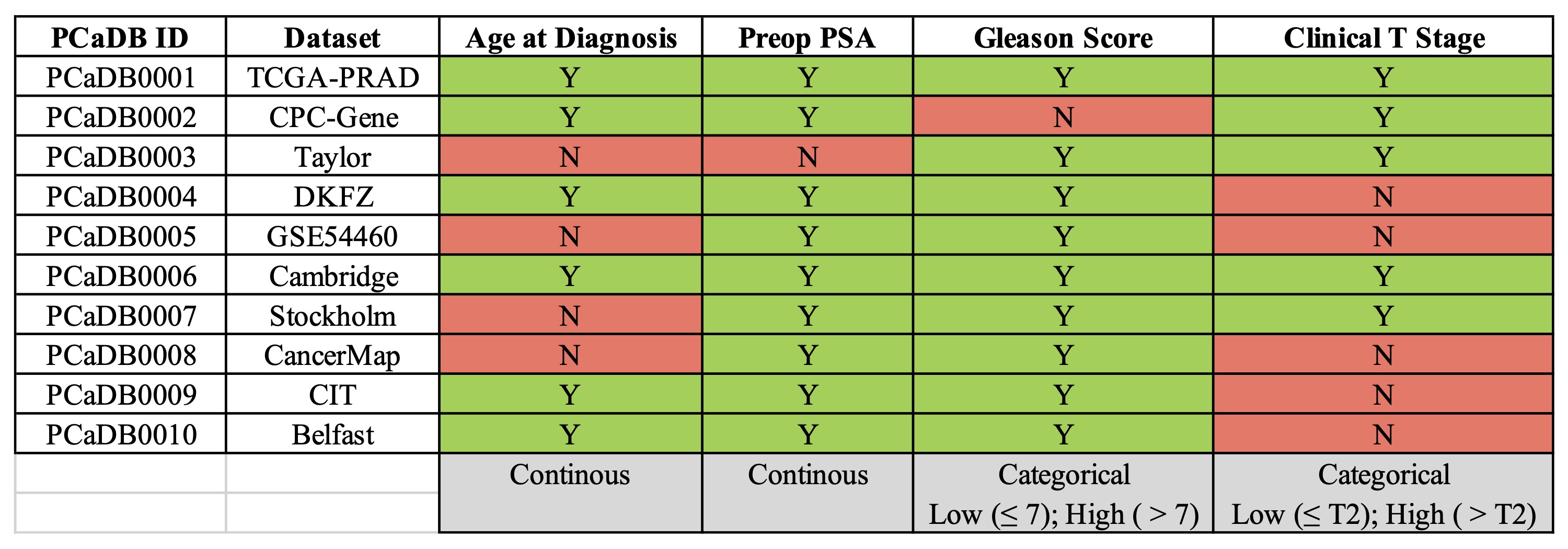
Multivariate Cox Proportional-Hazards (CoxPH) survival analysis of relapse-free survival (RFS) can also be performed to identify biomarkers associated with BCR by adjusting for some of the most important clinical factors, including age at diagnosis, preoperative PSA, Gleason score, and clinical T stage. The clinical factors that are included in the multivariate CoxPH model for each dataset merely depend on the availablity of the data, which has been summarized in a table below (Figure 3-6). Please be noted that not all the samples in the selected dataset are used in the multivariate CoxPH survival analysis because of the existing of missing data for the four cliical factors.
Figure 3-6. Multivariate CoxPH survival analysis
3.6. Development and validation of a new prognostic model
In PCaDB, an advanced functional module is provided, allowing users to provide a list of genes (e.g., genes that are significantly associated with the endpoint based on univiarate and/or multivariate CoxPH survival analysis), and select a survival analysis method, including multivariate CoxPH, Cox model regularized with lasso penalty (Cox-Lasso), or ridge penalty (Cox-Ridge), to develop and independently validate a prognostic model using the 10 datasets with the time to biochemical recurrence (BCR) data.
The prognostic model is trained using the selected dataset based on the selected survival analysis method. The R package
survivalis used to build the CoxPH model, and the R package
glmnetis adapted to build the Cox-Lasso and Cox-Ridge models with the penalties alpha (α) = 1 and alpha (α) = 0, respectively. Cox-Lasso uses L1 regularization technique, which adds “absolute value of magnitude” of coefficient as penalty term to the loss function, whereas Cox-Ridge uses L2 regularization technique that adds “quared magnitude” of coefficient as penalty term to the loss function. The major difference between Cox-Ridge and Cox-Lasso regression is that Cox-Lasso tends to shrink coefficients of the insignificant features to absolute zero, while Cox-Ridge never sets the coefficients to absolute zero. When training a Cox-Lasso or Cox-Ridge model, the tuning parameter lambda (λ), which controls the overall strength of the L1 or L2 penalty, is determined based on a built-in 10-fold cross-validation. A maximum of 1000 iterations is implemented over the data for all lambda (λ) values.
The risk score for a patient in the training set is calcualted as a linear combination of the gene expression valuesand coefficients of the signature genes, i.e., risk score = β1*E1 + β2*E2 + ... + βn*En, where β1 to βn are the coefficients of the signature genes and E1 to En are the normalized gene expression values in log2 scale. The median value of the risk scores for all patients is used as the threshold to dichotomize these patients into low- and high-risk groups. A KM plot is generated to show the prognostic performance of the signature in the training set. The R package
survivalis used to estimate the hazard ratio (HR) and 95% confidence intervals (CIs). The log-rank test is performed to compare the two survival curves and calculate the p value. Theoretically, any prognostic models should be significantly associated with the endpoint in the training dataset. Therefore, it's very criticial to perform external validations of the prognostic models in multiple independent cohorts. In PCaDB, the risk scores are calculated for patients in each of the nine remaining datasets with RFS data, to validate the prognostic model, and a forest plot is generated to show the HRs, 95% CIs, and log rank test p values from KM analyses in the nine validation datasets (Figure 3-7).
* Please be noted that only genes that are present in the training dataset are used for prognostic model development. If a gene in the final model has not been quantified in the validation dataset, the expression value would be set to zero.
Figure 3-7. Development and validation of the user-provided prognostic signature
Data Download
4.1. Download processed data
All the processed data deposited in PCaDB, including the
ExpresionSetof a transcriptomics data in the .RDS format, prognostic signatures in the .xlsx format, and gene annotation in the .RDS format can be donwloaded directly by clicking the link to the data on the Download page (Figure 4-1).
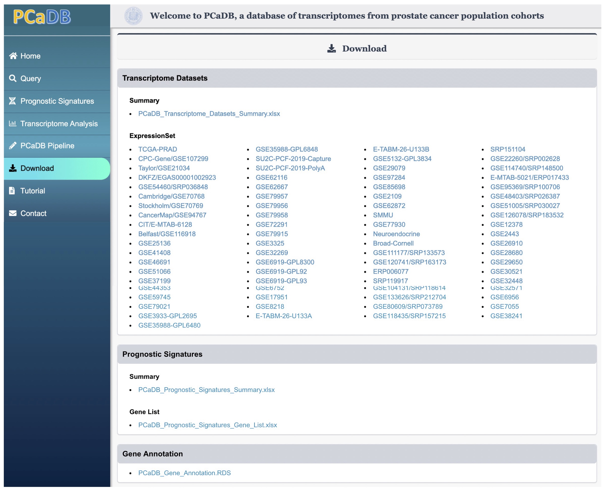
Figure 4-1. Download processed gene expression data, sample metadata, and gene annotation data
For example, suppose the .RDS file for the TCGA-PRAD dataset has been downloaded, the gene expression data and sample metadata can be easily retrieved by running the following command in R (Figure 4-2).

Figure 4-2. Retrieve gene expression data and sample metadata from the eSet object
4.2. Export data analysis & visualization results
We provide two download buttons (
PDFand
CSV) under each figure generated by PCaDB, allowing the users to download the high-resolution publication-quality vector image in PDF format and the data that is used to generate the figure in CSV format.
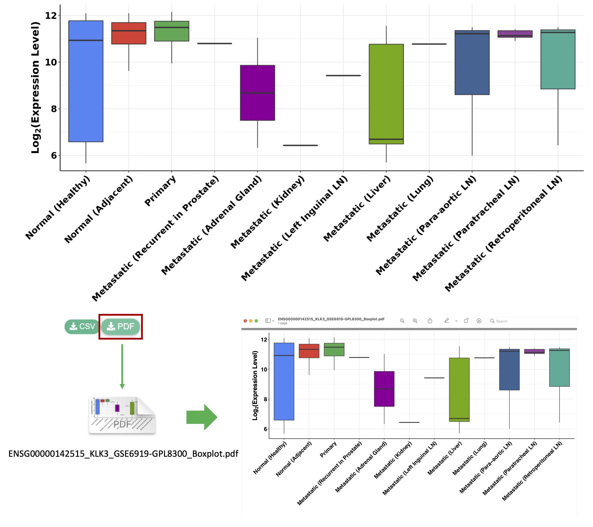
Figure 4-3. Download the publication-quality vector image in PDF format
In this example, the expression data of the selected gene
KLK3for the samples in the selected dataset GSE6919-GPL8300 will be saved to the CSV file
ENSG00000142515_KLK3_GSE6919-GPL8300_Expression.csvby clicking the download button (Figure4-4).
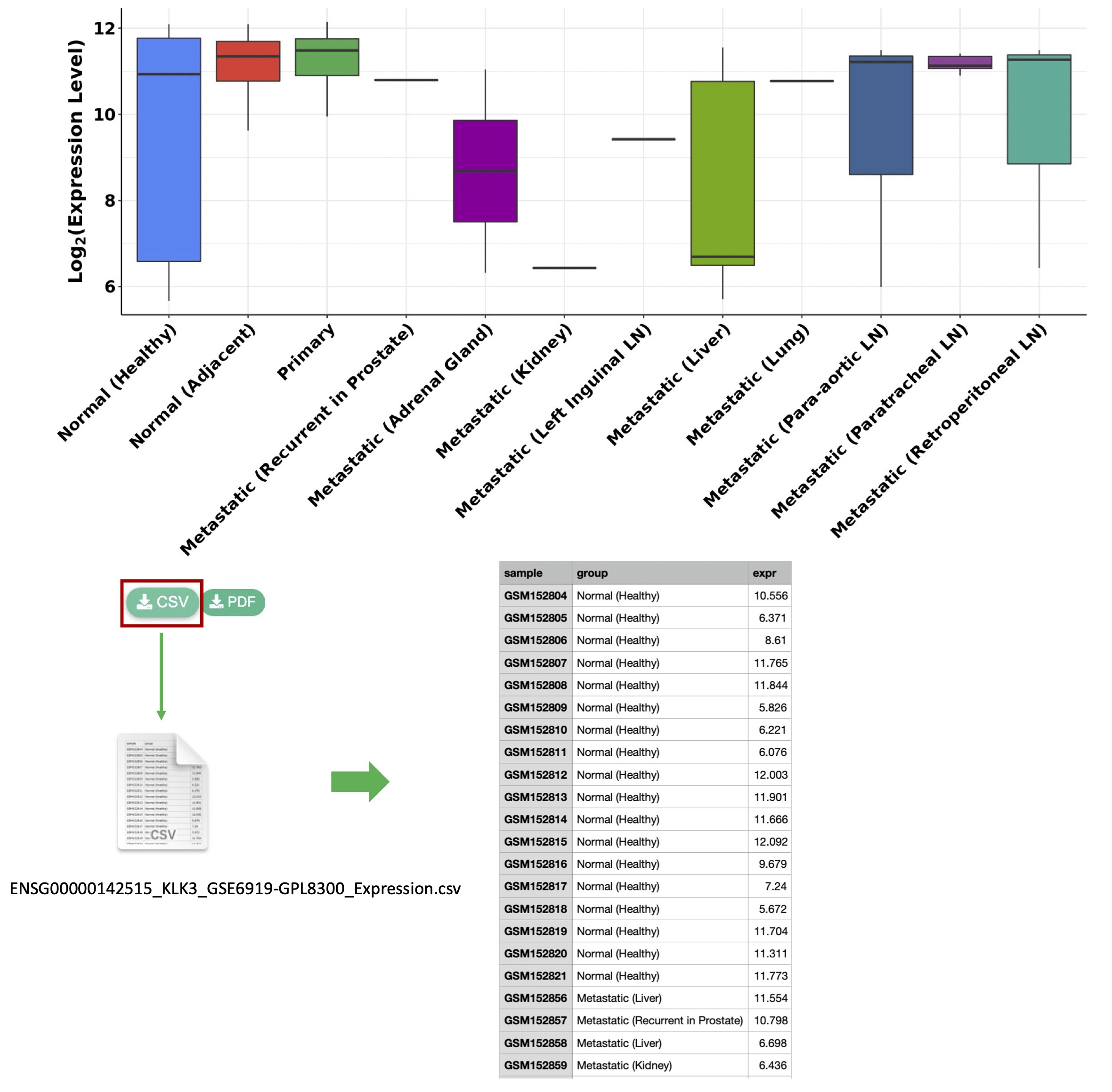
Figure 4-4. Download the data that is used to generate the figure to a CSV file
All the data tables generated for the data analysis outputs are also exportable in
CSVor
EXCELformats. The output can also be copied to the clipboard.